Creating an Automated Players Comps Worksheet

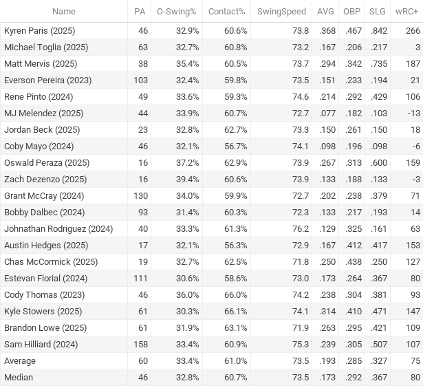
When analyzing players, I want more than a one-line projection, I want a range of possible outcomes. The problem with comps is that they are time-intensive. Once the worksheet is setup, a person can select and download the desired output in a few seconds. Here is the outputted table from the example procedure explained below.

A link to the sample spreadsheet is found here.

While I’m looking at a certain subset of stats, the procedure could be used for any comparison.

Disclaimer #1: While I’ll answer some questions in the comments for a few days, I don’t have time to create or fix anyone’s project. I’m not trying to be an ass but a working framework and example have been provided. Users can spend some working through their own kinks in the process. I sure did.

Disclaimer #2: As far as I know, the setup ONLY works in Google sheets, not in Excel. The sheet needs to use the QUERY function to automate the output and that functionality is not available in Excel.

Pick A Lane

The first step might be the easiest or the hardest to finish; determine what information to compare. So far, I created comps for projections, playing time, pitch types, and hitter skills. The list is endless.

In this instance, I wanted to compare a hitter’s core traits (power, eye, ability to make contact) to the actual outcome of similar players. Since it has been a short season so far, I included all available swing speed seasons (2023 to 2025).

Collect Information

The next step is to collect the information. The two preferred sources of information are FanGraphs and Baseball. The reason is that they included unique IDs for each player (MLBAMID). These IDs make it easy to match information for each player and not have to worry about similar names or different spellings.

For this sample, I wanted to use the limited available swing speed values from Baseball Savant with some plate discipline values from Fangraphs to find the actual stats for similar players, including playing time.

At FanGraphs, I downloaded this page. I copied the data and pasted it into the PlateSkills sheet.

The information from Savant needs a little data manipulation. I could not find a way to download the bat speed info by player and year. Instead, I downloaded each year (2023, 2024, 2025) and pasted each into the sheet BatSpeed. After pasting each dataset, the year is added to column S.

Combine Values Into One Sheet

After collecting all the information, the desired information was moved to one sheet. I picked the sheet from FanGraphs (PlateSkills). The reason is that it contains the player’s name, season, and team. A column needs to be created with all three because of the Max Muncy’s of the world. Sometimes the year doesn’t need to be included if only a single season is used. In column Q, the three values are combined using CONCATENATE with the following formula:

=concatenate(M7,” (“,A7,”, “,C7,”)”)

Next, the values from other sheets need to be combined. In this instance, the Bat Speed values aremoved from BatSpeed to PlateSkills. In both sheets, the MLBAMID (unique ID given to each player) and year are combined again using CONCATENATE (Column P in PlateSkills, column T in BatSpeed).

To bring the values from one sheet to another, use XLOOKUP. XLOOKUP will be one of the two key functions for setting up this sheet. An understanding of it is needed for several parts of the sheet. It has three components

XLOOKUP (ID used to find in another column, Column to find ID, Column with return value)

Here is the XLOOKIP code used for Cell R7 of sheet PlateSkills to find the bat speed value in BatSpeed.

XLOOKUP(P7,BatSpeed!T:T,BatSpeed!F:F)

The first value is the combined MLBAMID and season in Column P of PlateSkills. The next value in the same formula in the column in BatSpeed (column T). Finally, the bat speed is collected from column F.

Because of small samples or missing data, some players didn’t have bat speed values. For them, I used the league average value (71.17 mph). An IFERROR statement is used to get around this problem. It determines if there is an error (missing value) and then substitutes another value (league average value).

=IFERROR(XLOOKUP(P7,BatSpeed!T:T,BatSpeed!F:F),71.17)

Next, a new sheet needs to be created (‘+’ sign in lower left corner of sheets) and named (SwingDecisionComps). In the new sheet, select a cell near the top (B3), go to Data -> Data Validation -> click on Add Rule -> select Dropdown (from a range) -> under Dropdown (from a range), select the range which is PlateSkills, Column Q -> press Done. Now the hitter’s name and year can be selected from the cell.

The selected hitter’s values to be compared are added after the name to SwingDecisionComps using XLOOKUP. For example, the plate appearances are added to C3 with the following code:

=XLOOKUP($B3,PlateSkills!$Q:$Q,PlateSkills!F:F)

This is done with each of the compared values.

Compare Columns Using Z-Scores

To compare the columns, z-scores are used. Here are simple written and verbal explanations of z-scores.

The reason to use z-scores is that it takes variables of different data types like plate appearances (count), Contact% (percentage), and bat speed (mph) and puts them on the same comparable scale.

Note: While I won’t show the process, one other option besides z-score is to convert all the values into percentiles. The key is to get all the values on the same scale.

Find the Standard Deviation for the values in question. This is done for Columns F, G, H, and R in PlateSkills.

The variation for the selected player is calculated. In Row 2, Column T to W, the values are linked from SwingDecisionComps for the selected player. In Row 3, the standard deviation values are linked under the corresponding value.

Next, the combined difference from the selected player to everyone else is calculated. This is done by finding the absolute value of the z-score of each player. The absolute z-score is used because the total difference is needed, not the directionality. Here is the code for the first cell (T7).

=ABS(F7-T$2)/T$3

The ‘$’ sign locks in the player’s values when comparing to everyone else. The absolute standard deviation can then be calculated for the other categories (Column U to W) using the same process

Finally, the four values are added together in Column X

Note: The absolute standard deviations are weight the same here. The different columns can have different weights by using a multiplier.

Create the Final Display Sheet

Going back to the SwingDecisionComps sheet, it’s time to set up the money cell. The desired information will be transposed with one cell QUERY (B10). Here it is:

=QUERY(PlateSkills!$A$8:$X$1735,”select Q, F, G, H, R, I, J, K, L order by X limit 20″)

The first section of the function is ALL the data that could be displayed, in this instance, every cell with information in the PlateSkills sheet (PlateSkills!$A$8:$X$1735). Select all the data. Having all of it available makes future adjustments easier.

Next, the query needs to be written in quotes with the capital letter from each column put in the desired order. That code is followed by ‘order by X limit 20′. This code takes the 20 players with the closest stats to the selected player. Besides the compared stats, I brought over the players’ triple slash lines and wRC+.

Some notes on using QUERY

• On the query, the CAPITALIZATION of the columns matters.
• No other information can be in the cells, or there will be an error.
• If the range contains blanks, the blank values might get queried in the output.
• If the selected player is NOT to be included in the list, add where X > 0 after the L.

=QUERY(PlateSkills!$A$8:$X$1735,”select Q, F, G, H, R, I, J, K, L where X > 0 order by X limit 20″)

With these comps, feel free to change the number of them. Find the Average, Median, or range of outcomes.

One other item I added to the sheet is a downloadable Table. This can be found at Insert->Chart->in the dropdown Chart Type select Table Chart. The table’s functionality is funky and performs a few functions on its own. I like that I can set one up, change the player, and immediately download the table (select the table -> click on three dots in upper right-hand corner -> Download Chart -> select desired image type).

Wrapup

While the setup takes a little work, it requires no maintenance once set up, besides updating data. Also, once a player is selected, their results are immediately available. Hope you find the procedure and possible outcomes useful.