Much like Hot Right Now, Cold Right Now will be a weekly Ottoneu feature, primarily written by either Chad Young or Lucas Kelly, with a focus on players who are being dropped or who maybe should be dropped in Ottoneu leagues. Hot Right Now will focus on players up for auction, players recently added, and players generally performing well. Cold Right Now will have parallel two of those three sections:
- Roster Cuts: Analysis of players with high cut% changes.
- Cold Performers: Players with a low P/G or P/IP in recent weeks.
There won’t be a corresponding section to Current Auctions because, well, there is nothing in cuts that correspond to current auctions.
Roster Cuts
Ian Hamilton, Add% (7 days) – 29.49%
Sad news for Hamilton on the injury front has a lot of managers dropping him from their teams. Hamilton worked his way into the crowded closer committee in New York, but may now be out for a month or more. That 12.27 K/9 and a 1.23 ERA really had managers thinking they made the waiver claim of the season. Wise managers will find another reliever with save prospects to claim, they probably won’t keep him and stash him on the IL.
John Schreiber, Leagues with a Cut (7 days) – 28.85%
I don’t know what a “right teres major strain” is but it must be the reason Schreiber is being dropped. Schreiber had an 11.12 K/9, but a 4.24 BB/9 in 17 IP this season before his injury. Many managers were likely adding him because he probably would have accumulated holds and wins. He only has one win on the season but he does have six holds and last season, he had 22 holds. The smart move would be to cut him and find another reliever who is consistently lined up for hold opportunities. Going to the Steamer Rest of Season (ROS) projections page can help you identify some of those relievers who may be worth adding.
Hayden Wesneski, Leagues with a Cut (7 days) – 22.68%
Four home runs given up in his last appearance sent him back down to AAA. This is to be expected with a young pitcher, Wesneski is only 25. In eight starts, Wesneski gave up 10 home runs and he’ll have something to work on while he’s back at Triple-A Iowa. I don’t have anything else to write because Eric Longenhagen and Tess Taruskin have already written it:
“Nothing about Wesneski’s stuff suggests his early 2023 swoon will continue; his slider’s movement is identical to 2022 and still projects as a plus pitch, the best of a repertoire that should enable him to be a stable fourth starter. Even though the early results at Wrigley have not been good, there’s no reason to come off of Wesneski’s long-term projection.”
Alek Thomas, Leagues with a Cut (7 days) – 17.63%
Headed back to AAA, Thomas will, “work on fixing [his] swing while he’s in the minors[.]” He had a rough time against lefties batting .028. Against righties, he hit .273 with five doubles, two triples, and two home runs. But he and you and his coaches probably don’t want such a talented athlete to be isolated to only batting against right-handed pitchers. Esteban Rivera recently wrote a great piece about swing adjustments that really encapsulated Thomas’ issues with big-league pitching. Keeping him or cutting him in Ottoneu leagues is very dependent on where you currently find your team in the standings.
Wade Miley, Leagues with a Cut (7 days) – 15.71%
RotoWire reported that Miley, “is likely to be sidelined 6-8 weeks” due to a lat/rib injury. It’s difficult to keep an injured 36-year-old on your fantasy team, but Miley has produced a sub-3.50 ERA in his past two seasons and currently has a 3.67 ERA. He’s been steady and reliable, but managers will have to make a tough call when it comes to using an IL spot or not.
Cold Performers
Player stat lines reflect last 14 days among players with at least 20 PA in that time frame.
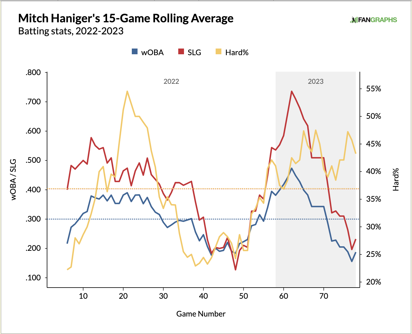
Mitch Haniger: 40 PA, .200/.200/.250, 1.18 P/G
With only 76 AB on the season as a whole, Haniger is still trying to get things going after
But, he may be starting to turn a corner as he has eight hits in the last 14 days, six singles, and two doubles. In that time period he 32.5% of the time and walked 0% of the time. That wouldn’t be so bad if he was hitting home runs in between. There is some reason to believe he could be on the cusp of a breakout. Take a look at his actuals vs. Statcast expected numbers in 2023:
AVG: .211 xAVG: .244
SLG: .329 xSLG: .418
wOBA: .240 xwOBA: .291
In addition, he’s hitting the ball hard, and if he continues to put the ball in play, he should see his stats come up. But, he’ll need to add some walks and home runs to make fantasy managers really be bought back in.
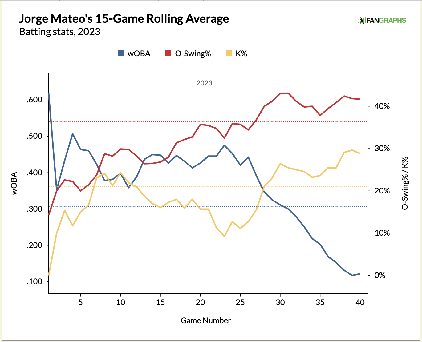
Jorge Mateo: 38 PA, .083/.105/.083, -1.09 P/G
This is a rough slump after starting the year so hot. The first month of the season shows that it wouldn’t be smart to drop Mateo. He can get hot and when he does it is absolutely electric. Right now, however, times are tough. The frustrating part about rostering Mateo is that in times like this when you make the very pertinent decision to leave him on your bench, he’ll find his way on base and steal every bag between him and home plate.
Jordan Montgomery: 10.1 IP, 0.89 P/IP
It’s odd to see Montgomery getting BABIP’d to shreds (.321) but with actuals and expected stats so closely in-line:
ERA: 4.21 xERA: 4.25
FIP: 3.82 xFIP: 3.97
Let’s compare Montgomery’s last three starts with his first six starts:
Jordan Montgomery Game Results Comparison 2023
| Games |
W |
L |
IP |
K/9 |
BB/9 |
HR/9 |
BABIP |
HR/FB |
ERA |
FIP |
xFIP |
| Last Three |
0 |
2 |
16.1 |
8.82 |
2.76 |
2.76 |
0.333 |
23.8% |
6.06 |
6.41 |
4.48 |
| First Six |
2 |
4 |
35.0 |
8.23 |
2.06 |
0.26 |
0.315 |
3.0% |
3.34 |
2.61 |
3.73 |
Home runs have really gotten to him in his last three starts where he gave up five total. When nearly of quarter of your fly balls go for home runs, there could be an issue. However, he’s still keeping his walks down, his BABIP is high across both time frames and he’s striking batters out. HR/9 is volatile and if Montgomery, or the wind, can find a way to keep balls in the yard, Montgomery should level out to what we expect from him as a fantasy starting pitcher.
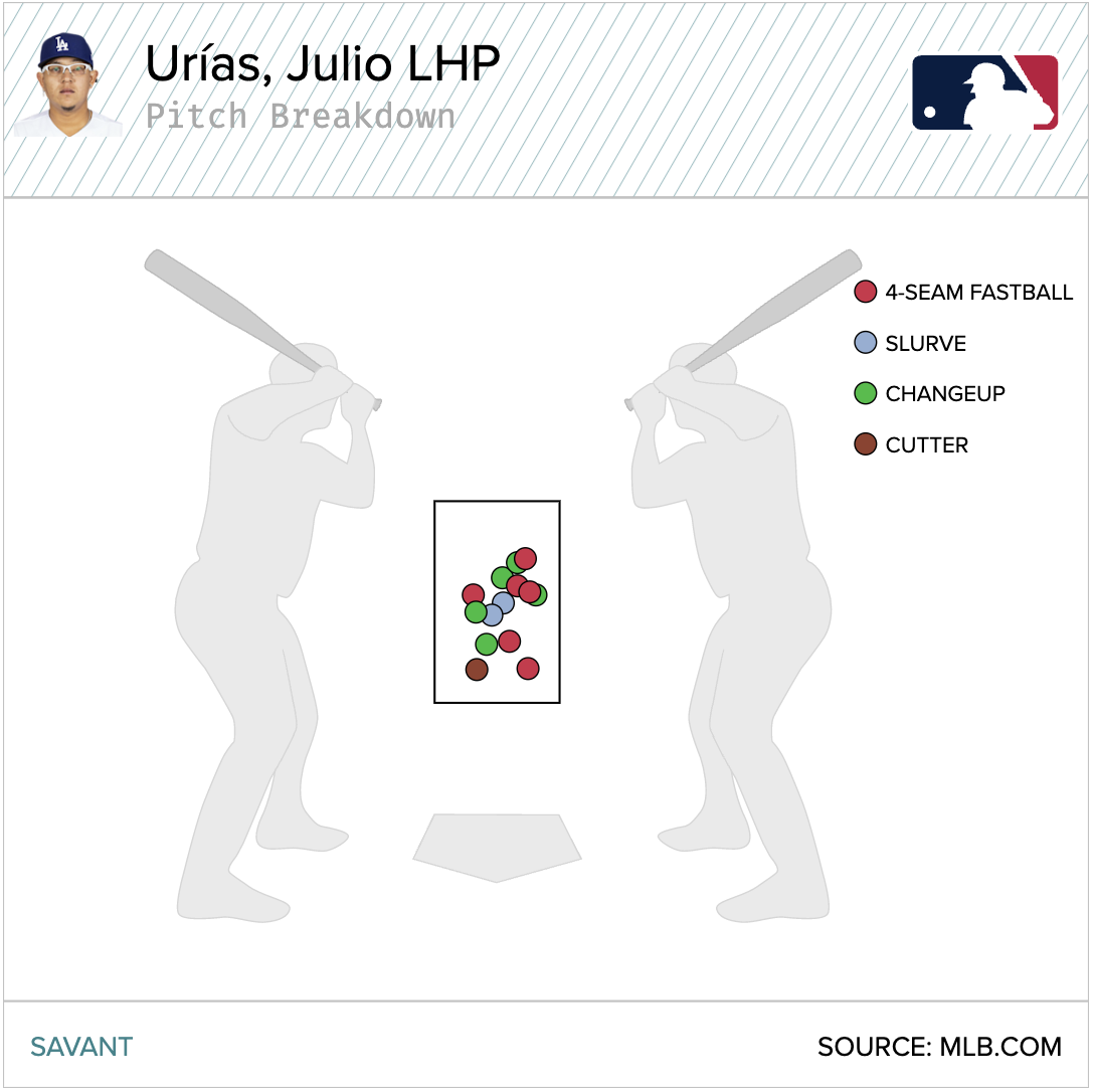
Julio Urías: 10 IP, 1.9 P/IP
According to RotoWire News, “Urías was placed on the 15-day injured list by the Dodgers on Saturday with a left hamstring strain” and perhaps some time to re-group and rest up will help the Dodgers lefty get back on track. He’s currently sporting a 4.39 ERA and a 4.37 xERA. Urías has a home run issue in 2023. So far, he’s given up 2.28 HR/9, he’s given up 14 so far this year, and he was projected by THE BAT, the projection system that gave him the highest mark, to give up 1.46 HR/9. There have certainly been a few changeups hung up in the zone. According to PitcherLists’ “loLoc%” which details the location of pitches low of the batter, Urías’ changeup is at 58.8% when the league is at 66.9%. The same thing is happening to his curveball or slurve, depending on which pitch identifier you’re looking at, where he is locating it low 52.5% of the time compared to the league average of 62.0%. In Ottoneu points leagues where home runs really hurt, Urías hasn’t been the pitcher most expected him to be, but he’ll come around.